The use of ensemble forecasting and data assimilation has made apparent the importance of local predictability properties of the atmosphere in space and in time (e.g., Toth and Kalnay, 1993, Molteni and Palmer, 1993). The “spaghetti” plots and other methods used to display operational ensemble products frequently show simultaneous high predictability in some areas and low predictability in others. The regional loss of predictability is an indication of the instability of the underlying flow, where small errors in the initial conditions (or imperfections in the model) grow to large amplitudes in finite times. The stability properties of evolving flows have been studied using Lyapunov vectors (e.g., Alligood et al, 1996, Ott, 1993, Kalnay, 2001), singular vectors (e.g., Lorenz, 1965, Farrell, 1988, Molteni and Palmer, 1993), and, more recently, with bred vectors (e.g., Szunyogh et al, 1997, Cai et al, 2001).
Bred vectors (BVs) are, by
construction, closely related to Lyapunov vectors (LVs). In fact, after an
infinitely long breeding time, and with the use of infinitesimal amplitudes,
bred vectors are identical to leading
Lyapunov vectors. In practical applications, however, bred vectors are
different from Lyapunov vectors in two important ways: a) bred vectors are
never globally orthogonalized and are intrinsically local in space and time,
and b) they are finite amplitude, finite time vectors. These two differences
are very significant in a very large dynamical system. For example, the
atmosphere is large enough to have “room” for several synoptic scale
instabilities (e.g., storms) to develop independently in different regions
(say, North America and Australia), and it is complex enough to have different
possible types of instabilities (such as barotropic, baroclinic, convective,
and even Brownian motion). Errico and Langland (1999) pointed out that bred
vectors are indeed different from LVs, and suggested that these differences
would be detrimental to the applications of bred vectors to ensemble
forecasting, a conclusion disputed in the response by Toth et al (1999). In
this paper we suggest that the local and finite amplitude properties of BVs
make them preferable to the use of LVs for both ensemble forecasting and data
assimilation. In section 2 we describe the construction of LVs and BVs. In section
3 we review the properties of BVs compared to LVs. In section 4 we indicate
that the number of bred vectors needed to describe the unstable growth of
perturbations is much smaller than the number of LVs with positive exponents
and provide a heuristic argument to explain this observation. Section 5 is a
brief summary.
2. Computation
of Lyapunov Vectors and Bred Vectors
Assume that we have an
evolving basic solution ![]() that satisfies the equations of a nonlinear model with a given
discretization in space and time integration scheme
that satisfies the equations of a nonlinear model with a given
discretization in space and time integration scheme ![]() . If the initial condition is perturbed, the linear evolution
of the perturbation is given by
. If the initial condition is perturbed, the linear evolution
of the perturbation is given by
![]()
where the matrix ![]() is the tangent linear
model (TLM) or propagator.
is the tangent linear
model (TLM) or propagator.
2.1 Computation of Lyapunov vectors
The leading Lyapunov vector is computed as follows:
1) Start with an arbitrary
perturbation ![]() of arbitrary size
of arbitrary size
2) Evolve it from ![]() to
to ![]() using the TLM
using the TLM ![]()
3) Repeat 2) for the
succeeding time intervals
After a sufficiently long
time ![]() , the perturbation
, the perturbation ![]() converges to the leading Lyapunov vector. The direction of
this vector is independent of the initial perturbation, the length of the time
interval
converges to the leading Lyapunov vector. The direction of
this vector is independent of the initial perturbation, the length of the time
interval ![]() or the choice of norm of the perturbation, properties not
shared by singular vectors. If during the repeated application of the TLM the
LV becomes too large it may be scaled down to avoid computational blow up.
Additional LVs can be obtained by the same procedure, except that after each
time step the perturbation has to be orthogonalized with respect to the
subspace of the previous LVs, since otherwise all the LVs would converge to the
leading LV.
or the choice of norm of the perturbation, properties not
shared by singular vectors. If during the repeated application of the TLM the
LV becomes too large it may be scaled down to avoid computational blow up.
Additional LVs can be obtained by the same procedure, except that after each
time step the perturbation has to be orthogonalized with respect to the
subspace of the previous LVs, since otherwise all the LVs would converge to the
leading LV.
2.2 Computation of Bred vectors
Bred Vectors (BVs) are computed as follows:
1) Start with an arbitrary
initial perturbation ![]() of size
of size ![]() defined with an
arbitrary norm. This initialization step is executed only once. The size of
defined with an
arbitrary norm. This initialization step is executed only once. The size of ![]() is essentially the
only tunable parameter of breeding.
is essentially the
only tunable parameter of breeding.
2) Add the perturbation to
the basic solution, integrate the perturbed initial condition with the
nonlinear model, and subtract the original unperturbed solution from the
perturbed nonlinear integration
![]()
3) Measure the size ![]() of the evolved
perturbation
of the evolved
perturbation ![]() , and divide the perturbation by the measured amplification
factor so that its size remains equal to A:
, and divide the perturbation by the measured amplification
factor so that its size remains equal to A:
![]() .
.
Steps 2) and 3) are repeated
for the next time interval and so on. It has been found that after a short
transient time of the order of the time scale of the dominant instabilities
(3-5 days for baroclinic instabilities, Toth and Kalnay, 1993, Corazza et al.,
2001a, a few months for a coupled ENSO model, Cai et al, 2001), the procedure
converges in a statistical sense. Additional bred vectors can be obtained by
choosing different arbitrary initial perturbations and following the same
procedure. Therefore all bred vectors are
related to the leading Lyapunov vector, since the additional BVs are never
orthogonalized. As discussed further in the next section, it has been found
that for global atmospheric models based on primitive equations or on
quasi-geostrophic equations, as well as for other strongly nonlinear models,
the bred vectors remain distinct, rather than converging to a single leading
bred vector, presumably because the nonlinear terms and physical
parameterizations introduce sufficient stochastic forcing to avoid such
convergence.
An alternative method is “self-breeding” (Toth and Kalnay, 1997). This approach, cost-free when performing ensemble forecasting, uses pairs of ensemble forecasts to generate the perturbation at the new time:
![]()
This difference is scaled down as before, and added
and subtracted to the analysis valid at ![]() . The two-sided self-breeding has the advantage that it
maintains the linearity of the perturbation to second order compared to the
one-sided generation of the bred vector which is linear to first order, but
otherwise the procedures produce similar results.
. The two-sided self-breeding has the advantage that it
maintains the linearity of the perturbation to second order compared to the
one-sided generation of the bred vector which is linear to first order, but
otherwise the procedures produce similar results.
3. Properties
of the bred vectors
Bred vectors share some of their properties with leading LVs (Corazza et al, 2001a, 2001b, Toth and Kalnay, 1993, Cai et al, 2001):
· Bred vectors are independent
of the norm used to define the size of the perturbation. Corazza
et al. (2001)
showed that bred vectors obtained using a potential enstrophy norm were
indistinguishable from bred vectors obtained using a streamfunction squared
norm, in contrast with singular vectors.
· Bred vectors are independent
of the length of the rescaling period as long as the perturbations remain
approximately linear (for example, for atmospheric models the interval for
rescaling could be varied between a single time step and 1 day without
affecting qualitatively the characteristics of the bred vectors.
· In regions that undergo
strong instabilities, the bred vectors tend to be locally dominated by simple,
low-dimensional structures. Patil et al., (2001) defined local bred vectors around a point in the 3-dimensional grid of the
model by taking the 24 closest horizontal neighbors. If there are k bred vectors available, and N model variables for each grid point,
the k local bred vectors form the
columns of a 25Nxk matrix B. The kxk
covariance matrix is C=BTB.
Its eigenvalues are positive, and its eigenvectors are the singular vectors of
the local bred vector subspace. The local effective dimension can be
measured by the Bred Vector dimension (BV-dim)
![]() ,
,
where ![]() are the square roots
of the eigenvalues of the covariance matrix. They showed that the BV-dim gives
a good estimate of the number of dominant directions (shapes) of the local k bred vectors. For example, if half of
them are aligned in one direction, and half in a different direction, the
BV-dim is about two. If the majority of the bred vectors are aligned
predominantly in one direction and only a few are aligned in a second
direction, then the BV-dim is between 1 and 2. The BV-dim attains its maximum value
k if all the bred vectors are
pointing in different directions. This happens either in quiescent regions,
where the amplitudes are small and there is little error growth, or after an
integration long enough to allow perturbations to become nonlinear and very
different from each other. Patil et al., (2001) showed that the regions with
low dimensionality cover about 20% of the atmosphere. They also found that
these low-dimensionality regions have a very well defined vertical structure,
and a typical lifetime of 3-7 days.
are the square roots
of the eigenvalues of the covariance matrix. They showed that the BV-dim gives
a good estimate of the number of dominant directions (shapes) of the local k bred vectors. For example, if half of
them are aligned in one direction, and half in a different direction, the
BV-dim is about two. If the majority of the bred vectors are aligned
predominantly in one direction and only a few are aligned in a second
direction, then the BV-dim is between 1 and 2. The BV-dim attains its maximum value
k if all the bred vectors are
pointing in different directions. This happens either in quiescent regions,
where the amplitudes are small and there is little error growth, or after an
integration long enough to allow perturbations to become nonlinear and very
different from each other. Patil et al., (2001) showed that the regions with
low dimensionality cover about 20% of the atmosphere. They also found that
these low-dimensionality regions have a very well defined vertical structure,
and a typical lifetime of 3-7 days.
· Using a Quasi-Geostrophic
simulation system of data assimilation developed by Morss (1999), Corazza et al
(2001a, b) found that bred vectors have structures that closely resemble the
background (short forecasts used as first guess) errors, which in turn dominate
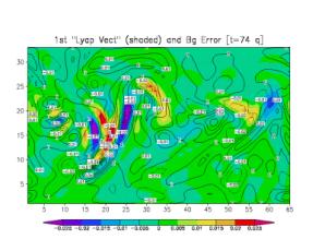
the local analysis errors (Fig. 2a). This structural similarity had been
conjectured by Kalnay and Toth, 1994 based on the qualitative similarity
between the analysis cycle and the breeding cycle. Corazza et al., (2001a)
showed that the background error has a very substantial projection into the
subspace of 10 bred vectors, with an angle less than 10o (a local
pattern correlation of 0.985 or more) in most areas. The angle became as large
as 45o only in some areas were the background error was very small.
· The number of bred vectors
needed to represent the unstable subspace in the QG system is small (about
6-10). This was shown by computing the local BV-dim as a function of the number
of independent bred vectors. Convergence in the local dimension starts to occur
at about 6 BVs, and is essentially complete when the number of vectors is about
10-15 (Corazza et al, 2001a). This should be contrasted with the results of
Snyder and Joly (1998) and Palmer et al (1998) who show that hundreds of
Lyapunov vectors with positive Lyapunov exponents are needed to represent the
attractor of the system in quasi-geostrophic models.
· The fact that only a few bred
vectors are needed, and that background errors project strongly in the subspace
of bred vectors, allowed Corazza et al (2001b) to develop cost-efficient
methods to improve the 3D-Var data assimilation by adding to the background
error covariance terms proportional to the outer product of the bred vectors,
thus representing the “errors of the day”. This approach led to a reduction of
analysis error variance of about 40% at very low cost.
4. Comparison of bred vectors and LVs
We have seen that BVs and LVs share some properties but also have significant differences, namely that BV are finite amplitude, finite time, and that they have local properties in space. These properties result in significant advantages of BVs for data assimilation and ensemble forecasting.
4.1 Finite amplitude, finite time
The fact that BVs have finite
amplitude provides a natural way to filter out instabilities present in the
system that have fast growth, but saturate nonlinearly at such small amplitudes
that they are irrelevant for ensemble perturbations. For example, Toth and
Kalnay (1993) found that with amplitudes characteristic of the analysis errors
for the geopotential height (between 1m to 10m), bred vectors grew by about 1.5
per day, and were similar to the NCEP operational bred vectors. With amplitudes
of the order of 1 cm, the bred vectors (dominated by convective instabilities)
grew 10 times faster and had maximum amplitude in the tropics. With even
smaller amplitudes, James Geiger (personal communication, 2001) has found
growth rates of the order of 50/day in a tropical primitive equations model.
These convective instabilities saturate at very small amplitudes. If the model
had enough resolution to include molecular motion, Brownian motion would
provide even faster (but clearly irrelevant) instabilities. As shown by Lorenz
(1996) Lyapunov vectors (and singular vectors) of models including these
physical phenomena would be dominated by the fast but small amplitude
instabilities, unless they are explicitly excluded from the linearized models.
Bred vectors, on the other hand, through the choice of an appropriate size A of the perturbation, provide a natural
filter based on nonlinear saturation of fast but irrelevant instabilities.
4.2 Local versus global representation
The local representation of BVs results in a reduction of the number of modes needed to represent a field of growing errors in the initial conditions, compared to LVs obtained by global orthogonalization. We now present a heuristic argument with a simple example of a system containing three independent regions of instability (denoted A, B and C in Figure 1). Assume that in each of them there are two unstable modes or shapes that have a similar growth rate and are therefore equally probable, one with total wave number 1 (a single high or low) and one with total wavenumber 2 (a high and a low). From a local point of view, only two bred vectors are needed to represent all possible local combinations (since each local area has two possible modes). For example, the first two bred vectors in the figure are enough to represent all possible local structures. On the other hand, the number of independent global shapes is
n = (2´2)3 – 1 = 63,
given that there are two modes in each of the three areas, and each of them can have either a positive or a negative sign. Therefore, with global orthogonalization we would need 63 global Lyapunov vectors to capture all possible directions. If we increase the number of local independent areas and/or the number of dominant modes, the number of global degrees of freedom increases very rapidly, whereas the probability of capturing all local independent shapes with a small number of bred vectors n decreases very slowly.
4.3 Comparison of BVs and LVs
As mentioned before, a
comparison of the bred vectors with the forecast errors that dominate the
analysis errors in the QG simulation system shows that they have very similar
characteristics. Fig. 2a shows this similarity between the background error
(contours) and an arbitrary bred vector (shaded) chosen as the leading LV (Fig. 2a). Every bred vector is
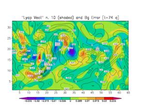
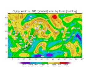
qualitatively similar to the leading LV. Figs. 2b and 2c show the same
background error (contours) with the 10th and 100th LVs
superimposed (shades). The successive LVs are obtained by orthogonalizing after
each time step with respect to the previous LVs subspace. The orthogonalization
requires the introduction of a norm and we have chosen the square of the
potential vorticity norm. As a result, the successive LVs have larger and
larger horizontal scales (a choice of a streamfunction norm would have led to
successively smaller scales in the LVs). Beyond the first few LVs, there is
little qualitative similarity between the background errors and the LVs.
Summary
In a system like the atmosphere with enough physical space for several independent local instabilities, BVs and LVs share some properties but they also have significant differences. BV are finite amplitude, finite time, and because they are never globally orthogonalized, they have local properties in space. Bred vectors are akin to the leading LV, but bred vectors derived from different arbitrary initial perturbations remain distinct from each other, instead of collapsing into a single leading vector, presumably because the nonlinear terms and physical parameterizations introduce sufficient stochastic forcing to avoid such convergence. As a result, there is no need for global orthogonalization, and the number of bred vectors required to describe the natural instabilities in an atmospheric system is much smaller than the number of Lyapunov vectors with positive Lyapunov exponents. The BVs are independent of the norm, whereas the LVs beyond the first one do depend on the choice of norm.
These properties of BVs result in significant advantages for data assimilation and ensemble forecasting for the atmosphere. Errors in the analysis have structures very similar to bred vectors, and it is found that they project very strongly on the subspace of a few bred vectors. This is not true for either Lyapunov vectors beyond the leading LV, or for singular vectors unless they are constructed with a norm based on the analysis error covariance matrix (or a bred vector covariance). The similarity between bred vectors and analysis errors leads to the ability to include “errors of the day” in the background error covariance and a significant improvement of the analysis beyond 3D-Var at a very low cost (Corazza, 2001b).
References
Alligood K. T., T. D. Sauer and J. A. Yorke, 1996: Chaos: an introduction to dynamical systems. Springer-Verlag, New York.
Buizza R., J. Tribbia, F.
Molteni and T. Palmer, 1993: Computation of optimal unstable structures for
numerical weather prediction models. Tellus, 45A, 388-407.
Cai, M., E. Kalnay and Z.
Toth, 2001: Potential impact of bred vectors on ensemble forecasting and data
assimilation in the Zebiak-Cane model. Submitted to J of Climate.
Corazza, M., E. Kalnay, D. J.
Patil, R. Morss, M. Cai, I. Szunyogh, B. R. Hunt, E. Ott and J. Yorke, 2001:
Use of the breeding technique to determine the structure of the “errors of the
day”. Submitted to Nonlinear Processes in Geophysics.
Corazza, M., E. Kalnay, DJ
Patil, E. Ott, J. Yorke, I Szunyogh and M. Cai, 2001: Use of the breeding
technique in the estimation of the background error covariance matrix for a
quasigeostrophic model. This volume.
Errico, R. and R. Langland,
1999: Notes on the appropriateness of bred modes for generating perturbations
used in ensemble forecasting. Tellus, 51A, 442-449.
Farrell, B., 1988: Small
error dynamics and the predictability opf atmospheric flow, J. Atmos. Sciences,
45, 163-172.
Kalnay, E 2001: Atmospheric
modeling, data assimilation and predictability. Chapter 6. Cambridge University
Press, UK. In press.
Kalnay E and Z Toth 1994:
Removing growing errors in the analysis. Preprints, Tenth Conference on
Numerical Weather Prediction, pp 212-215. Amer. Meteor. Soc., July 18-22, 1994.
Lorenz, E.N., 1965: A study
of the predictability of a 28-variable atmospheric model. Tellus, 21, 289-307.
Lorenz, E.N., 1996:
Predictability- A problem partly solved. Proceedings of the ECMWF Seminar on
Predictability, Reading, England, Vol. 1 1-18.
Molteni F. and TN Palmer,
1993: Predictability and finite-time instability of the northern winter
circulation. Q. J. Roy. Meteorol. Soc. 119, 269-298.
Morss, R.E.: 1999: Adaptive
observations: Idealized sampling strategies for improving numerical weather
prediction. Ph.D. Thesis, Massachussetts Institute of Technology, 225pp.
Ott, E., 1993: Chaos in
Dynamical Systems. Cambridge University Press. New York.
Palmer, TN, R. Gelaro, J.
Barkmeijer and R. Buizza, 1998: Singular vectors, metrics and adaptive
observations. J. Atmos Sciences, 55, 633-653.
Patil, DJ, BR Hunt, E Kalnay,
J. Yorke, and E. Ott, 2001: Local low dimensionality of atmospheric dynamics.
Phys. Rev. Lett., 86, 5878.
Patil, DJ, I. Szunyogh, BR
Hunt, E Kalnay, E Ott, and J. Yorke, 2001: Using large member ensembles to
isolate local low dimensionality of atmospheric dynamics. This volume.
Snyder, C. and A. Joly, 1998:
Development of perturbations within growing baroclinic waves. Q. J. Roy.
Meteor. Soc., 124, pp 1961.
Szunyogh, I, E. Kalnay and Z.
Toth, 1997: A comparison of Lyapunov and Singular vectors in a low resolution
GCM. Tellus, 49A, 200-227.
Toth, Z and E Kalnay 1993:
Ensemble forecasting at NMC – the generation of perturbations. Bull. Amer.
Meteorolo. Soc., 74, 2317-2330.
Toth, Z and E Kalnay 1997:
Ensemble forecasting at NCEP and the breeding method. Mon Wea Rev, 125,
3297-3319.
Toth, Z., I Szunyogh and E
Kalnay, 1999: Response to Notes on the appropriateness of bred modes for
generating perturbations used in ensemble forecasting. Tellus, 51A, 442-449.